Should you give a job offer to the candidate you’ve just interviewed or keep searching? Stop for gas or look for a cheaper gas station? Marry the person you’re with or keep dating?
With some details abstracted, these problems share a similar structure. The goal is to pick the best option from a pool whose size is roughly known, where the options are evaluated one at a time and you can’t go back to a previously rejected choice. The general form of his is called the “secretary problem“, after a formulation of the problem where secretary candidates are interviewed in succession. The general solution to the secretary problem is to go through the first 1/e (37%) of candidates, then choose the next one that is higher ranked than all of the previous options.
The “secretary algorithm” picks the best option at least 37% of the time, the last option 37% of the time (in cases where the single best choice came in the early group and set the bar too high), and a pretty good option the remaining times. Can we improve on this?
The secretary algorithm only uses an ordinal ranking of the options: which option is best, second-best, etc. But in all real-life examples, we often have a cardinal measure for each option as well. We can grade interviewees on a rubric or a test, we see the price of gas in each station, we use Putanumonit’s decision matrix guide to rate potential partners [1].
We’ll use the example of my dating life in New York to look for a better algorithm. This example will use gendered language; although secretaries come in all genders, people I’ve dated have all identified as the same one.
For illustration purposes, here are the retrospective spreadsheet scores for the first 20 women I went on dates with in New York: 4.9, 6.2, 5.8, 8.1, 4.8, 6.5, 5.1, 7.2, 5.2, 4.5, 4.9, 5.5, 5.3, 5.9, 4.8, 6, 5.5, 6.5, 5, 7.8. Reminder: these scores measure only someone’s compatibility with me, which is driven mostly by the kind of weird person I am. This is not an assessment of anyone’s objective value as a unique and beautiful human being.

This chart [2] suggests a probability distribution of potential partner compatibility, not just an order ranking. The go-to probability distribution on Putanumonit is a normal bell curve, but it seems like a poor fit here – the distribution is clearly skewed with the majority on the left and a single tail of high scorers on the right side. Also, the tails of a normal distribution drop off very quickly, going as 
Let’s try the exponential distribution. It’s single-tailed, easy to work with, and a lot more romantic with a drop-off rate of 

The formula for the exponential distribution density is simply the decaying exponential function: 

In my data, the mean is 5.8 and the standard deviation is 1, so in our model, the distribution will start from 5.8 – 1 = 4.8, ignoring the single outlier lady who snuck in below that point (I must have been drunk). The distribution density is 
Here are some consequences of this model:
, so 70% of the women I meet will score between 4.8-6 on compatibility.
- Only 1 in 25 will score above 8, and only 1 in 67 will score above 9. Romance is hard.
- If I keep meeting women in the 5-6 range, it shouldn’t cause me to update the model a lot. If start regularly meeting women who score below 4.8 or above 7.5, it’s a sign that the model is way off and I should reassess.
If I feel like I have 34 more dates in me, the secretary algorithm would advise me to stop fooling around after the 20th date (


To come up with a better algorithm given the actual distribution, we can use induction to make the optimal decision at each step.
- If I’m down to my last date, I have to be happy with whatever I get – the average is 5.8.
- If I’m on the penultimate date, I will reject anyone below 5.8 (since I know I can get that on average on my last try) and accept anyone above that. The average of scores above 5.8 is 5.8+1 = 6.8. The chance of finding someone above 5.8 is, conveniently,
Thus, my expectation on the penultimate date is
.
- Let’s assume we’ve calculated that if I’m down to n dates left, my expected outcome is an. Thus, on the nth-to-last date, I will accept someone above an and reject someone below an. The chance of seeing a score above an is
and if I do, their average score is an+1. So my expectation with n+1 dates left is
. With this sequence rule, we can start from the last date and calculate an for each n.
Here’s my expectation as a function of the number of dates I have left.
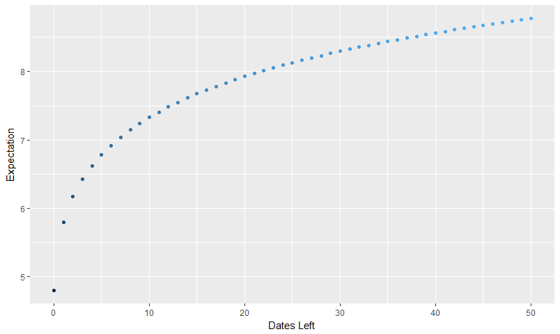
Let’s see how this “exponential secretary” algorithm does compared to the regular one.
With 34 dates left, my expectation is 8.4, up from 8.14. Great success! However, the new algorithm says that if I keep dating unsuccessfully my standards should go down. When I’m down to 24 dates left, I dip below the original secretary algorithm threshold of 8.1. When I get into the single digits, my willingness to settle should increase, well, exponentially [4].
My standards can also go up! If I improve my OkCupid skills and start going on dates with more compatible partners (7s and 8s instead of 5s and 6s), I should refit the model and get a distribution with a higher mean. This will raise my expectations, as it should.
The biggest difference between the algorithms concerns meeting someone amazing early on in the process. The original secretary algorithm rejects all the early candidates regardless of how good they are. If instead of 34 dates I had 180 dates left, it would tell me to ignore all candidates before the 74th one (1/e = 74/200) no matter how exceptional. The exponential secretary algorithm is more lenient. If I have enough data points to nail down the model and I meet someone who’s a huge positive outlier (like a 10 on my scale) I should go for it regardless of the number of potential candidates remaining. I strongly endorse this conclusion.
In summary, here’s what you can do to improve on the secretary algorithm for secretary problems:
- Obtain a cardinal measure of the candidates, not just a rank order. If no obvious measure presents itself, putanumonit anyway.
- After a few data points have been gathered, plot them to see if they fall in a reasonable distribution that you can model. Err towards distributions with fatter tails, since you don’t want the model to exclude possible points that are outside the initial range of data.
- Once you have a distribution, you have a cumulative probability function: the chance of meeting a candidate who scores above some threshold.
- By induction from the last candidate, you can estimate the expected score you can achieve based on the number of candidates left. The expectation at n candidates left is your threshold at n+1.
- As you gather more data, keep refitting the model, especially if the data points fall far outside the predicted pattern.
- At times you will feel regret and desire to call a secretary you have rejected a few months ago. Don’t. She has moved on and is happier without you.
Footnotes
[1] When the marriage question popped up on Reddit, a link to my decision matrix post popped up within an hour of a link to the secretary algorithm wiki page. As a reminder, the point of decision matrices is to allow you to think of many values and variables at once, not to replace all of them with a single arbitrary number.
[2] The R code I used to generate these charts is on my Github.
[3] One of the cool things about the exponential distribution is that the truncated distribution looks exactly the same, just with a different starting point. So if my exponential distribution has a mean and deviation of theta and I truncate it to only look at points above a cutoff Y, the resulting distribution will have the same deviation and a mean of Y+theta.
[4] There are some very entertaining online debates about settling in romance, but I’m certainly not wading into those right now, just doing some math.

“Gender.” The word you’re looking for is “sex.” The people you’ve dated have all been the same sex. Female.
LikeLike
Gender is what people associate with pronouns. If his point was to preemptively defend against complaints of pronoun discrimination, gender was the right word to use.
LikeLike
Nah. I bet the sex was different with each one.
LikeLiked by 2 people
The post is well taken. The point that finding the correct probability distribution to use can improve one’s ability to predict future and, more specifically, how to do so is well taken. There is still the question of whether or not one is using the correct probability distribution. Is there a way to determine this conclusively? There isn’t a method (that would apply to any situation with fitting parameters) that I know of but evidence can be found.
I have used the <a href=”http://en.wikipedia.org/wiki/Akaike_information_criterion” rel=”nofollow”>Akaike Information Criterion corrected (AICc) to test for how good the exponential model for Mr. Falkovich’s data is. I made a visualization of the compatibility scores that I will use to help illustrate the fitness of models to this data. It includes a better histogram of the scores then Mr. Falkovich used in his post as well as the Empirical Distribution Function for the compatibility scores.
Ideally, I should chose my method of analysis before I know what the data is. I was not able to follow this advice this time. After reading the post, I speculated that the log-normal distribution would be a good fit. This was from visualizing the data and because I can come up with an explanation for why the compatibility values would be distributed thusly.
On the surface, it seems like a <a href=”http://en.wikipedia.org/wiki/Normal_distribution” rel=”nofollow”>normal distribution would work. A decision matrix takes a linear combination of different values and a sum of different random (or close enough) independent values produces a normal distribution regardless of probability distribution is for each variable. The issue is that, in this case, the variables are likely not independent. I would guess that, say, “20,000 Wednesdays,” and “Building a Future,” would be correlated for each person.
A more complicated model would be, (underlying characteristics)->(superficial characteristics)->(measured traits)->(compatibility score). In this sense how the underlying characteristics combine to produce the superficial characteristics should ultimately determine the basic nature of the distribution in compatibility score (though not necessarily the specific final distribution). If this is dominated by simple addition then this would yield a normal distribution. If instead, this is dominated by simple multiplication then this would yield a log-normal distribution.
(I want to point out that in the above paragraph, I use superficial in a denotative sense: that is the superficial characteristics are the characteristics that can be directly observed. The underlying characteristics are opaque and can only be guessed at from indirect information. I do not intend superficial in the common connotative sense in that I think plenty of superficial characteristics can be deep and meaningful.)
I can buy that this process is either largely addition, largely multiplication, or something more complicated. As the data does not look symmetrical (and looks to me like it would be a good candidate for a log-normal fit), I guessed the log-normal distribution would fit better than an exponential distribution. An exponential distribution is used to model things like how long a DMV transaction takes (not including the wait time which would not follow an exponential distribution) or the different lengths between successive road-kill caucuses on a highway. I don’t see any reason why scores for how compatible a person is in marrying Jacob would follow such a pattern.
Before I do calculations there is a big problem. To use the AICc, I need to calculate the likelihood function for each model I use. The exponential distribution is zero for numbers smaller than the starting point. This would yield a likelihood of 0 for the exponential model as there is a data point for a number smaller than the starting point. I need to figure out how to deal with that.
I spent a bit of time going over different ways to handle that single data point. I don’t want to ignore inconvenient data points as that is horrible form but there isn’t any good way of handling this issue in this problem that I know of. I decided to break up the data into two different distributions concatenated together, an exponential distribution for the data points above the zero point and another exponential distribution for the data points below the zero point. I then weight each distribution in proportion to how many data points are above and below the zero point so to keep the probability that any value is found to be 1. This, unfortunately for the exponential model, increased the degrees of freedom from 2 (the standard deviation and the zero point) to 4 (two standard deviations, the zero point, and the weighting).
Also, since Mr. Falkovich wisely has not released details of his decision matrix, I do not know if the scores have to come out to a multiple of 0.1 or if he rounded the scores to the nearest tenth. Since the probability distributions I am considering are all continuous probability distributions, I should integrate each distribution from 0.05 below to 0.05 above the given data point. I did the lazier thing and multiplied the value of the probability distribution by 0.1 for the value of each data point. I think that this won’t affect anything of my analysis but I haven’t done to work to show this.
First, the result for the exponential distribution. I used the measured standard deviation of about 0.99 and the measured starting point (the mean less the standard deviation) of 4.78 to start and to define the exponential distribution above the starting point. I used the measured mean (as there is only one point) of 4.5 for the data less than the starting point and the difference between this and the starting point of about 0.28 as the standard deviation for the exponential distribution bellow the starting point. Finally the lower distribution is multiplied by 1/20 and the upper by 19/20 in proportion to the number of points above and below the starting point.
This yields a likelihood of getting the exact distribution of values of about 3.1 x 10^-13. That’s pretty good for 20 data points. This yields an AICc of about 68.27 (lower AICc’s are better). This shows the <a href=”//imgur.com/F7TKUf9” rel=”nofollow”>PDF of the fit and the CDF of the fit. The exponential model looks like it fits the data very well (look at the CDF as compared with the EDF).
I compare this to the standard normal distribution using a measured mean of about 5.78 and measured standard deviation of about 0.99. The PDF and <a href=”//imgur.com/U8S3EHq” rel=”nofollow”>CDF can be found in these links. It doesn’t look like it fits as well as the exponential and, indeed, the likelihood with the normal model is about 1.4 x 10^-14 with an AICc of about 68.55.
Then there is the log-normal distribution with a measured mean of the natural logarithms of the values of about 1.74 and a standard deviation in the natural logarithms of the values of about .16. The PDF and CDF can be found in these links. To me it looks like the log-normal fits the data better than the normal (which shouldn’t be a surprise) but not as well as the exponential. As it shows, the likelihood for the log-normal model is about 5.3 x 10^-14 which is in-between the two. It, however, has the lowest AICc so far of about 65.82. It seems as though the extra fitting parameters of the exponential model I used has made the log-normal model more attractive.
As a sanity check, I test a uniform model with a minimum of 4.5 (the smallest data point) and a maximum of 8.1 (the largest data point). The PDF and especially the <a href=”//imgur.com/DXYWmVY” rel=”nofollow”>CDF shows this not to be a good fit. However it has the second highest likelihood so far of about 1.8 x 10^-13 and highest AICc so far of about 63.38.
It may be natural to wonder why such a bad fit has such a high likelihood and that is because models which can fit the minimum and/or maximum of the model tend to have artificially high likelihood values. The uniform model analyzed gives a 0% chance to finding any compatibility score lower than 4.5 or higher than 8.1 of anybody that Mr. Falkovich would have been willing to date. The other distributions are open ended on two ends. The fitted uniform model states that slightly more extreme values then have already occurred cannot happen while the other models have to consider a non-zero probability of ludicrously extreme values. This problem is not unique to the uniform model (it would exist if I fitted a beta distribution to the model) but it is still of value to test it.
Lastely, after looking at why the models gave the scores they gave (I discuss this a few paragraphs later), I tested a fitted <a href=”//en.wikipedia.org/wiki/Gamma_distribution” rel=”nofollow”>gamma distribution using a zero point of 0. I chose parameters that maximized the likelihood function and got a shape parameter of about 36.7 and a rate parameter of about 6.36. Here are the PDF and CDF comparisons. This gives a likelihood of about 3.6 x10^-14 and an AICc of about 66.61.
From the AICc’s one can find the relative probability that a model is the correct model for the data if the only things known are the data, the likelihood that the particular model would find that particular data, and the number of fitting parameters. A model with a relative probability of 0.4 would be half as likely from this limited information as a model with a relative probability of 0.8. Other information (such as the feasibility of a model or how the model was chosen) should mater but is not measured with this test.
Here is a summary of the results:
Model (number of fitting paramiters): likelihood; AICc; relative probability
Uniform (2): 1.82×10^-13; 63.38; 1.00
Log Normal (2): 5.35×10^-14; 65.83; 0.294
Gamma fitted (2): 3.61×10^-14; 66.61; .198
Exponential (4): 3.11×10^-13; 68.27; .0867
Normal (2): 1.37×10^-14; 68.55; .0752
Why these models give the values they give is instructive. The uniform model is simple: for any value in its range it gives a 2 7/9 % (about 2.78%) chance of choosing that value. All the other four models give comparable numbers until the final three values (7.2, 7.8, and 8.1) when the probabilities of getting these values drops to less than 1.5% for getting 7.2 in any of the other models and less than .35% for getting 8.1 in any of the other models. It seems that Mr. Falkovich’s desire is fulfilled and the drop off for higher scores is not as severe as the normal (or any of the other models including the exponential) would predict.
Mr. Falkovich is wrong in that the exponential model is better because of behavior at the tails. The normal model, the log-normal model, and the gamma model give higher probabilities to getting 7.2 and 7.8 then the exponential model gives. It’s only in the 8.1 data point does the exponential model give a higher probability then the other models and this is where the probability is very low anyways.
The exponential model gives the highest likelihood because of behavior in the low range. The exponential model gives about a 9.5% chance of getting a value of 4.8 which is the highest of any data point for any model. The other models don’t start giving higher probabilities until the 5.8 data point where the normal, log-normal, and gamma functions all start doing so. The exponential distribution may be the best model of those tested but because of how well it does in predicting the relatively low scores, not its ability to predict relatively high scores (unless someone wants to date more than a hundred people).
Looking at why the uniform model wins is instructive. All of the models tested (including the exponential distribution) fall off too quickly for higher values to be believable. A distribution that does not fall off as quickly would fit better. As the gamma distribution can have different end behavior, I decided to test that (though without fitting for the zero point of the gamma distribution as this can skew the results as talked about with the uniform distribution). A beta distribution would be better but without knowing what maximum and minimum bounds to use it would show an artificially low AICc and is a mess to fit properly when fitting these bounds and didn’t want to bother.
In the end I do not believe that an uniform model is a good model (both because it visually fits so poorly and because there is good reason to believe that it is wrong). None of the relative probabilities are really all that bad. In this situation, analyzing things qualitatively as well as quantitatively, I would say that I don’t know what the true distribution is. Such comparable relative probabilities suggests that one cannot differentiate between the tested models solely on goodness of fit anyways.
I should point out that if I keep the relative likelihood of my exponential model but incorrectly set the number of fitting parameters to 2, then that model would win. I made a choice on how to adjust that model for the 4.5 value and making different choices could very well change what rank this model makes. I doubt any reasonable choice would find that model being a clear winner or clear looser amongst the models chosen to be tested but it is reasonable that someone would come to slightly different fine grain conclusions then I did.
I should point out that I am not a professional at data analysis. I am very much an amateur and do this for fun. I hope that if you’ve reached the end then you have gotten some value out of my discussion but I caution you not to trust my methods or claims I have made without some other supporting evidence. If you actually know what you’re doing and spotted an error of mine (major or minor) then please let people where know. I did all calculations and created all visualizations in Microsoft Excell Home 2013 32-bit version 15.0.4953.1000 except for finding the fit parameters for the gamma model used in which I did the calculations in Octave version 4.2.2. I hope I got all of the formatting in this comment correct.
Post Script: Now that I am ready to post this I have a desire to test a beta distribution with a lower bound of 0 and an upper bound of 10. This is because I am guessing that this is the maximum and minimum possible values that the decision matrix could create. I’ve already written everything up and don’t want to spend time rewriting it or delaying in publishing. I don’t want to be scooped.
LikeLike
Argh, all of links are broken. They include an extra quotation mark at the end. Delete this and they should work.
LikeLike
You can learn about including inline links using WordPress markdown here.
LikeLike
Why exponential rather than lognormal? Lognormal seems to be a better intuitive fit; while most people in the world are not going to be good fits, the low end of the distribution should be reserved for people who are not just bad fits but actively bad, someone who is selected for getting along with you as badly as possible.
LikeLike