I’m struggling a bit with the next post in the dating sequence. I can’t put any numbers in it, only some pretty personal stories and questionable ideas that touch on touchy subjects. I’m really not sure I should even write it. That leaves me with two options:
- Not write it.
- Before I write it, scare my entire readership away with a 4,000 word mathematical geek out about a 30 year old research paper, that’s going to include a Monte Carlo simulation of 320,000 jump shots.
If you know me at all, you know this isn’t much of a dilemma.
This post is tagged rationality because it deals with biases in decision making. It’s also tagged defense against the dark arts: we’re going to see how even good research papers get statistics wrong sometimes, and how smart statistical skepticism when scrutinizing science studies can save your skin.
Who Has the Hot Hand?
Steph Curry hits a 3 pointer, the crowd cheers. The next trip down the floor he hits another, from the corner. The buzz in the building rises in pitch, another shot with a hand in his face… swish! The crowd is standing now, screaming, everyone feels that Curry is on fire. “The basket is as big a barn door to Steph now,” the announcer is giddy, “He can’t miss!” Curry catches the ball at the top of the arc and releases another three pointer, the ball curves smoothly through the air. There’s no way he’s going to miss, is there?

The hot-hand fallacy is the intuitive tendency to assume that people will continue to succeed after a row of successes, even when success and failure come from a random process. It was was explained in Gilovich, Vallone and Tversky in 1985, who concluded that there’s no evidence for “hot hands” or “streak shooting” actually happening in basketball. They classified the belief as a fallacious heuristic – a mistaken judgment. The publication followed a stunning string of groundbreaking papers on heuristics and biases by Amos Tversky, who won the Nobel Prize later for his work with Daniel Kahnemann. I guess everyone just kinda assumed that Tversky’s hot streak must keep going and he can’t be wrong on this one.
Gamblers vs. Streakers
The first weird thing about the hot-hand fallacy (HHF) is that it’s supposed to be the same thing as the gambler’s fallacy (GF), except with precisely the opposite outcome. Gambler’s fallasticians believe that a coin that landed heads several times in a row is more likely to land on tails on the next flip because it’s “due”. GF really victimized the roulette players who kept betting on red when the wheel landed on black 26 times in a row in Monte Carlo in 1913. Wouldn’t it have actually made sense for these gamblers to switch to “hot hand betting” and double down on black? Besides being the intuitive thing to do after seeing 20 blacks in a row, pure Bayesian rationality would also seem to point that way. My prior on the roulette wheel being broken to bias black is not large, but it’s larger than 1 in 1,000,000. 1 in a million is less than the odds of seeing 20 spins on the same color in a row with a fair wheel. After 20 blacks, I wouldn’t be going back.
Supposedly, both GF and HHF come from the representativeness heuristic: people don’t believe a 50-50 variable should have long streaks of one outcome because heads-heads-heads-heads-heads doesn’t look like a fair coin. If the coin is known to be fair, people believe that the next flip “must” land tails to make the streak more “fair like” (GF). If the “coin” is actually Steph Curry, people decide he’s not actually 50-50 to hit his next shot but rather that he morphed into a 90% shooter (HHF). So: GF for objects and HHF for people.
But wait, do people expect Steph to continue hitting 90% for the rest of his career? Of course not! After a single miss everyone will assume he’s back to 50-50. I’m still not sure how, according to the theory, people decide if they’re going to HHF and assume a Curry basket or GF and assume he’s due for a brick. Maybe they flip a fair coin to make up their mind.
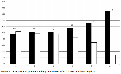
Croson and Sundali (2005) figured out how to expense a fun weekend to their research grant and took a trip to a Nevada casino to see the fallacies in action. Gambler’s fallacy with actual gamblers is a slam dunk: after six spins on the same color, 85% of roulette players bet the other way. The sample size isn’t huge, but the data seems unequivocal:
The evidence for hot hand abuse is a bit slimmer.
Croson and Sundaly: Of our 139 subjects, 80% (111) quit playing after losing on a spin while only 20% (28) quit after winning. This behavior is consistent with the hot hand; after a win players are likely to keep playing (because they’re hot).
The information above is utterly useless without knowing the base rate of winning on a spin, if 10% of spins won it would mean than people quit more after winning! I figured out that number from other data in the paper: it’s 33% (1024 / 3119). Also, 100% of the times someone quits because they ran out of chips happen after a losing spin. How many of the people who quit did so because they lost their last chip? If it’s more than 13% (the difference between the 67% who lost their last spin and the 80% who quit after losing), the conclusion isn’t only annulled, but reversed.
Spoiler alert: research papers that contain the data of their own refutation is going to be a theme today. Stay tuned.
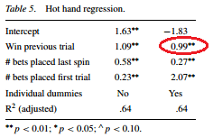 The main support for the hot hand effect comes from this regression on the right. People who just won place 1 additional bet, 12 on average instead of 11, when controlling for bets placed on the first and previous spins. The researchers couldn’t directly observe the amounts, just the number of different bets, and used that as a proxy. Obvious counterargument is obvious, Croson and Sundaly make it themselves:
There are alternative explanations for these behaviors. For example, wealth effects or house money effects might cause an increase in betting after a win. In our empirical data we will not be able to distinguish between these alternative explanations although previous lab experiments have done so.
When people are doing something weird, I often prefer to assume irrationality rather than conjuring convoluted utility functions to explain away the behavior (can I call that the Economist’s Fallacy?) In this case, however, putting one extra bet after having won seems quite reasonable. That’s how you would bet if, for example, you were trying to manage risk in order to play for a fixed number of spins and then get lunch. Whatever you think of the rationality level of people spending their day at the roulette table, it’s really hard to see much hot-hand fallacy there.
Shooters Gonna Shoot
Bocskocsky, Ezekowitz and Stein (2014) couldn’t get a trip to Vegas approved, so they went back to basketball armed with some great data that wasn’t dreamt of in 1985: cameras that track each player and the ball every second of the game. Without the distraction of Vegas, the researchers first developed a full model of shot difficulty that incorporates everything from the angle of the nearest defender to the time remaining in the game.
Armed with that model, the paper shows that “hot” players take slightly more difficult shots (e.g. from further away and in the face of tighter defense). Controlling for difficulty, players do shoot better after a few makes but not enough to make up for the increased difficulty. However, if a player who just made two shots takes another one of the same difficulty fans are right to expect a 2.4% better chance of sinking the shot compared to a player coming off two misses.

The bottom line is, the study is excellent but not very exciting. It concludes that the hot-hand isn’t a fallacy while also calculating that players are better off shooting less after a streak. Fans are justified to expect a hot streak to continue if they adjust for shot difficulty, but not if they don’t.
Finally, the Andrew Gelman-shaped Angel of Statistical Skepticism (ASS) on my shoulder reminds me to watch out for beautiful gardens that hide many forking paths. Even being completely honest and scrupulous, the researchers have a lot of small choices to make in a research project like this. Which of the dozens of variables to include in assessing shot difficulty? Which measures of “heat” to focus on? Which parameters to include the regression? Every choice makes perfect sense in the moment, but the fact is that those choices were available. A slightly different data set could have pushed the researchers towards doing a slightly different analysis that would’ve found statistical significance for some other result. A tiny effect size plus a multitude of “researcher degrees of freedom” make me think that the 1% p-value on the main finding is probably no better than a 5%, and 5% p-values are wrong at least 30% of the time.
I think that Bocskocsky, Ezekowitz and Stein did a great job and I certainly don’t believe they were in any way dishonest, but I’d be very happy to bet at 100-1 odds that their 1% p-value will not replicate.
The Hot Hand Bias Bias
Why even spend hours fitting models to data when you can do some arithmetic and turns other people’s data against itself? Miller and Sanjurjo (2015) did just that, and almost made $200,000 off a hedge fund guy while at it.
Miller and Sanjurjo noticed that even for a perfectly random variable, any limited sequence of observation is likely to show an anti-hot-hand bias. This confounds attempts to detect hot hands and contributes to the gambler’s fallacy. For illustration, lets look at sequences of 3 basketball shots. We assume that every player hits 50% of their shots, so each one of the 8 sequences is equiprobable. For each sequence (imagine it’s 8 players), we’ll calculate the percent of made baskets followed by another make.

We assumed that every player hits 50% of their shots no matter what, but somehow the average player makes 41.7% of their shots after a made basket! The discrepancy comes from the fact that 50% is averaged across all shots, but 41.7% is averaged across all players. Changing the aggregation or averaging level of your data can not only mess up your finding, but also flip it and reverse it.
If you bet against streaks continuing on the roulette, you will win most days but on the few days you lose, you’ll lose a lot. If, like Gilovich and Tversky, you look at a lot of basketball players, most players will appear to shoot worse after a streak but the few that shoot better will shoot much better. That better percentage will also continue over more shots since those players will have more and longer streaks.
Gilovich let 26 basketball players from the Cornell varsity teams shoot uncontested jump shots from a distance at which each players shoots 50%. He found an insignificant 4% increase in shooting after 3 makes vs. after 3 misses. Miller and Sanjurjo apply their correction to the original 1985 data, and calculate an implied difference of 13%!
The only question is, why apply corrections to poorly aggregated data when we can just change the aggregation level directly?
Data of Their Own Demise
To their credit, Gilovich, Valone and Tversky not only went out to the gym with the varsity teams (can you imagine Calipari’s Wildcats participating in a statistics study?) but also provided the full data of their observations and not just the percentages:
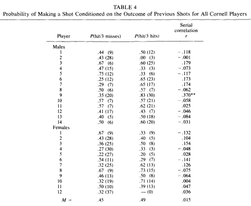
As we saw, averaging across all players finds a gap of 4% (49% vs. 45%) in shooting after a hot streak vs. a cold streak. The numbers in parentheses are the actual shots taken, using these along with the shooting percentages allowed me to reverse engineer the data and calculate total makes and misses after streaks.
- After 3 misses: 161 out of 400 shots = 40%.
- After 3 makes: 179 out of 313 shots = 57%.
That 17% is a humongous difference, equal to the difference in 2-point shooting between the second best player in the NBA this season and the fourth worst. The difference disappears in the original study because of aggregation levels. When you aggregate by players, the super-streaky Male #9 (48% gap) counts the same as his consistent friend, Male #8 (7%). However, dude #9 took four times as many post-streak shots as his buddy, when that data counts four times as much the shooting gap emerges clear as day.
Gilovich also looks at free throw shooting data by the Celtics and again goes to considerable lengths to avoid seeing evidence of hot-hand shooting:
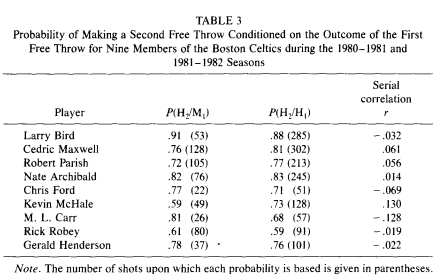
Gilovich starts by asking a bunch of supposedly ignorant and biased basketball fans to estimate the shooting percentage of a 70% average free throw shooter after a make and a miss. They estimate an average gap of 8%: 74% vs. 66%. Instead of looking at the gap directly, Gilovich calculates a correlation for each player, finds that none of them are significant, and happily proclaims that “These data provide no evidence that the outcome of the second free throw is influenced by the outcome of the first free throw” (Gilovich et al. 1985).
If you ask me, the evidence that the data provide is that players hit 428/576 shots after a miss (74.3%) and 1162/1473 after a make (78.9%) for a nice 4.6% gap.
Oh no, Gilovich objects, not so fast: “Aggregating data across players is inappropriate in this case because good shooters are more likely to make their first shot than poor shooters. Consequently, the good shooters contribute more observations to P (hit/hit) than to P (hit/miss) while the poor shooters do the opposite, thereby biasing the pooled estimates” (Gilovich et al. 1985).
Good point there, Dr. Gilovich, but remember that you asked the fans about 70% shooters specifically. We can avoid the good shooter/bad shooter bias by grouping players with identical FT%. As fate would have it, Paris, Ford, McHale and Carr all shoot between 70.5% and 71.2%: almost identical and close to 70% (I calculated each player’s exact shooting data from the number of shots and percentages in the table). These four players shoot 3.2% better after a make than after a miss.
Is a 3-4% gap significant? Who cares, the word “significant” is insignificant. A pernicious mistake that scientists constantly make is assuming that every rejection of the null is confirmation for the alternative. The fact that the data is unlikely under the null hypothesis doesn’t mean it’s any likelier under some other model. Here, Gilovich et al. make the flipped mistake: assuming that failure to reject the null hypothesis (0% gap after a make) confirms the null is true. However, the naive alternative (fan estimate) was an 8% gap. You can calculate p-values from now till the Sixers win, it doesn’t change the fact that 4% is as close to 8% as it is to 0%. The kind of statistical malpractice where a 4% result rejects the 8% hypothesis and confirms the 0% one is why some Bayesians react to frequentists with incandescent rage.
Rage aside, I’m left with a dilemma. On the one hand, disagreeing with Amos Tversky probably means that I’m not so smart. On the other hand, the Cornell students shot 17% better after a streak of makes and Tversky’s friends concluded “no effect”. Screw it, argument screens off authority: The hot-hand fallacy is dead, long live the hot hand!
The Streak is the Signal
Summary so far: research paper that claims that hot-hand shooting exists finds a 2% improvement in shooting after a streak, research paper that claims that hot-hands are bullshit finds gaps between 3% and 17%. Science FTW!!!
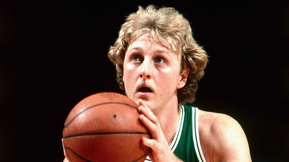
Even if the data was straightforward, it’s still just correlations and regressions. Without a plausible mechanism to explain the effect I trust it only as far as I can throw it. So why does hitting shots make you hit more shots? The announcers usually babble something about confidence or “being in the zone”, but I can’t throw announcers really far and I trust their analysis even less. If you’ve seen Steph Curry or Larry Bird shoot, you wouldn’t doubt that they’re 100% confident in every single shot they take.
It turns out there’s a remarkably simple answer that accounts for the hot-hand effect: all you need is a player having a priori different shooting percentages in different games. The simplest model assumes that each shot a player takes has the same odds of going in, but what if a player has games where something makes his shooting percentage higher or lower independently of streaks?
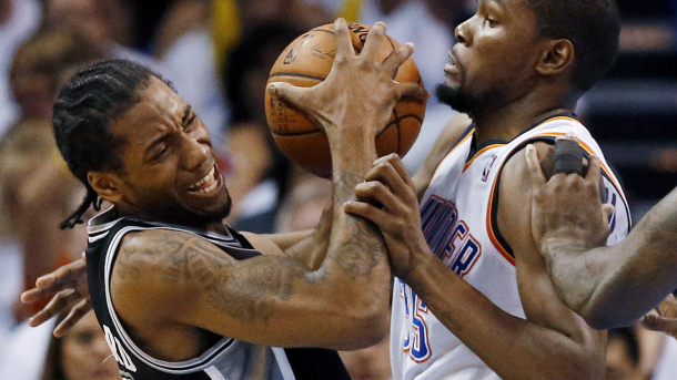
Let’s look at Kevin Durant, a dude who’s pretty good at shooting basketballs. He takes 20 shots a game and makes 50% of them over a season. In a specific game, however, Durant may have defensive player of the year Kawhi Leonard inside his shirt and shoot 32%. The next game, he’s guarded by octogenerian Kobe Bryant and something called Larry Nance Jr., he shoots 78%. Even if we assume that Durant’s shooting percentage doesn’t change throughout the game, in games where he shoots a higher percentage he’ll also get more streaks, and more attempts at shot-after-streak.
To see this in action, I simulated 1,000 games for Durant and counted the shots made and missed after 3 hits in a row. I simulated 20 shots in each game, but in 500 of them his shooting percentage is set to 60% and in the other 500 it’s set to 40%.
| # of Games | FG% | Streaks of 3 | Make after streak | Miss after streak | After streak FG% |
|
500 |
60% | 1872 | 1124 (60%) | 748 (40%) | 1333 / 2423 = 55% |
| 500 | 40% | 551 | 209 (38%) |
342 (62%) |
The chance of making a shot after a streak is either 60% or 40% depending on the game, but more than three quarters of the streaks happen in the 60% games. Every shot made after a streak gives another opportunity for a hot-hand shot, in a couple of the simulated games Durant makes 9 or 10 shots in a row! Because of that, even though his overall shooting percentage is exactly 50%, Durant’s shooting percentage after a streak is 55%. The fans are justified to expect a hot hand after 3 makes: the streak doesn’t cause the higher scoring chance, but it sends a signal that Durant is having a high FG% game. We have a perfect explanation for hot hands without any (hot) hand waving about “confidence” and “zones”.
Deviations of Deviations
The “variable shooting” theory is simple, elegant and explains the hot-hand shooting gap perfectly. Researchers take note: if you have a beautiful theory, don’t risk it by exposing it to ugly data! Oh, what the hell, I’m not getting paid for this anyway.
We can’t directly tell from someone’s shooting success what the underlying percentage was in a particular game, and we’re looking for evidence that the underlying percentage actually differs from one game to another. A consistent 50% shooter (no variability in underlying percentage) will still hit 3/9 on a bad day or 12/16 on a lucky outing. However, he’ll have less games where he shoots a number that’s very different from 50% than someone who alternates games with 60% and 40% underlying probabilities. We can find indirect evidence for game-to-game fluctuations by looking at how variable the game-to-game actual shooting percentage is. The higher the observed variance, the more evidence is shows for underlying variance. The question is, how much higher should it be?
A player’s field goals in a game follow a Binomial Distribution with parameters n=number of shots and p=underlying FG% for that game. The variance of a binomial variable is 

The leader in 2-point field goal attempts last season is LaMarcus Aldridge, who made 47.5% of his shots and took 18.45 attempts per game. If his underlying FG% was always 47.5%, the variance in his shooting percentage would be:

The standard deviation we would see over a season would be:


If instead of a steady 47.5% LaMarcus shoots either 10% above or below that number (57.5% in half his games and 37.5% in the other half), the variance would increase by 
Invariable Shooting
11.7% standard deviation in game-to-game FG% isn’t a perfect estimate of the actual variability because the number of shots a player takes changes each time and that pushes the variance higher. However, if a players underlying percentage goes up and down by 5% we still expect see about a 1% increase in game-to-game standard deviation relative to the baseline case in which he enters each game with a constant underlying FG%. To figure out that baseline, I looked at the top 10 players from last season in 2-point attempts (2PA) and simulated each of their seasons 20 times. For each game, I kept the actual number of attempts fixed but generated a random number of makes using the player’s season-long 2-point shooting percentage (2P%). All the data are from the magnanimous treasure trove of Basketball-Reference.com.
For example, Aldridge made 8 out of 24 shots (33%) on the last game of the 2015 season. His season long 2P% was still 47.5%, so in my 20 simulations he hit 9, 4, 9, 10, 7, 8, 14, 12, 12, 9, 12, 9, 10, 5, 10, 8, 9, 11, 6 and 12 of his 24 shots. I took the game-to-game shooting percentage deviation in each simulated season and averaged these to get the baseline deviation. I compared this to the player’s actual game-to-game deviation, I looked for the latter to be around 1% for most players.
| Player | 2P% | 2PA | Baseline Deviation | Actual Deviation | Baseline – Actual | 2PA-2P% correlation |
| LaMarcus Aldridge | 47.48% | 18.45 | 11.99% | 12.21% | 0.22% | .02 |
| Nik Vucevic | 52.42% | 16.22 | 13.05% | 11.28% | -1.77% | .17 |
| Anthony Davis | 54.00% | 17.46 | 12.73% | 15.82% | 3.09% | -.02 |
| Russ Westbrook | 45.82% | 17.66 | 12.79% | 12.62% | -0.17% | -.04 |
| Pau Gasol | 49.51% | 14.45 | 13.21% | 13.01% | -0.20% | .04 |
| Blake Griffin | 50.40% | 16.70 | 12.40% | 12.40% | 0% | -.16 |
| Monta Ellis | 48.69% | 13.54 | 14.35% | 16.62% | 2.27% | .12 |
| Boogie Cousins | 46.88% | 17.93 | 12.91% | 12.56% | -0.35% | -.10 |
| Marc Gasol | 49.95% | 13.02 | 14.40% | 12.06% | -2.34% | .32 |
| Ender Wiggins | 45.30% | 12.32 | 14.46% | 12.33% | -2.13% | .11 |
Shit, I really liked that theory.
Only 2 out of 10 players have actual game-to-game variance that’s significantly higher than the baseline, and 3 have a much lower one! Three explanations come to mind:
- I messed up the math or the simulation, you can spot the error and earn yourself a gift.
- Statistical coincidence, 10 players is a small sample, shit happens.
- Some mechanism is adjusting these players’ 2P% back to the mean within a game.
An example of #3 would be if players who start the game shooting well continue by taking more and worse shots, just like Bocskocsky saw happening after a streak. In fact, a high FG% game likely has streaks of makes after which the player will take bad shots and turn the high FG% game into an average FG% one. We can at least see evidence for these players shooting more often by looking at the correlation of their 2P% with attempts. Indeed, all three shoot more when they shoot well (right column).
Does that explanation sound plausible? That’s how bad science practice sounds like: alluring, seductive, and oh-so-reasonable. A post-hoc just-so story with little support in the data is still a crappy post-hoc just-so story if I came up with it myself. The bottom line is that I spent hours on that simulation and didn’t learn much of use, but I’ll be damned if I succumb to publication bias on my own blog.

Conclusion
Here’s what I learned from a week of digging into the dirt of hot hand research until my own hands got tired and bloody:
- Once we account for shot difficulty (or in cases like free throws where difficulty isn’t a thing), players shoot a bit (2%-4%) better after making a few shots in a row. Probably.
- Neither gamblers nor basketball fans are horribly confused by the “hot hand fallacy“, if they overestimate the chance of a successful streak continuing it’s not by much. Possibly.
- Science is hard. If you have a lot of analysis choices available, it’s very easy to let them lead you down a path of mirages. In the worst cases, your choice of analysis can lead you away from good conclusion (17% gap in Cornell!) and towards bad ones. Certainly.
Science – turns out it’s even harder than dating.

> Before I write it, scare my entire readership away with a 4,000 word mathematical geek out […]
At first, I misread this as “40,000 word” and got a little worried. I breathed a sigh of relief when I realized that it was actually a manageable size.
Thanks for blogging!
LikeLike
I’ve always understood streakiness to be defined as variance in the ability to accomplish the task whether it make a shot, get a hit, stop the on goal shot, what have you (that is if a player is considered to be on a roll, they are accomplishing their task more than they usually do). The analysis is complicated by how fine a player’s streakiness is. By looking at game to game results, streaks lasting shorter than a game will get lost in the analysis. Streaks lasting months could still be found by taking this measure.
I propose a way to measure a player’s streakiness. The measure is susceptible to the above limitation as I will show but can still have a use and can be used to answer questions. This assumes that a player has an underlying chance of success p. If streakiness exists, the number of times a player has a chance of success or failure (such as taking a shot) depends on their comparative success rate (such as taking more shots if they’re more likely to fall or more at bats if they’re getting on base more). This number will be normalized on the level the analysis is designed to catch (such as for each game). In this analysis, the game by game (or other analysis resolution) percentage will be taken for each player with each game being weighted the same and not dependent on the number of trials (in this example taking the fg% for each game and averaging them and not the total number of shots made divided by the total number of shots attempted for the season). Interestingly if streakiness exists, then the fg% for each player (and other similar statistics in Basketball or other sports) is likely to be higher than p because the games they take more shots (games they are better at shooting in) are weighted more when calculating the season total fg%.
Two things will influence a player’s chance of success in each game, the game to game variance, and improvements or decay of ability during the course of a season. Without a model for the later it is hard to adjust this statistic for that factor. It may be tempting to take an affine approximation and normalize game to game figures to this approximation and this would work with some models but for a model that stays mostly constant for most of the season and then they player gets significantly better or worse at the end (or beginning) of a season, the affine model will attribute more of the variation to increasing or decreasing skill then is warranted.
The method will assume that the player’s skills remain constant over the analysis period. Players who have their skills change significantly over this time will have their streakiness overstated with respect to other players but in a sense this change fits the definition of streakiness I have chosen. The player’s real success rate normalized to weight each analysis resolution the same will be taken to be p. This could be done, for example, by averaging each games fg% for the player in question over the course of a season.
In the simplistic case, if a player has a p+d chance of success in half of the analysis resolutions and p-d chance in half of the analysis resolutions then the variance will be expected to increase by d^2 from what it would be with a constant chance of success. This is shown by the following: in half of the n trails the result is increased by d and in the other half it is decreased by d. This does not change the average and the new variance of the new set is \sigma ^2 = \frac {1}{2} \sum_i \frac {2}{n} \left ( x_i + d – \bar {x} \right ) + \frac {1}{2} \sum_j \frac {2}{n} \left ( x_j – d – \bar {x} \right ) = \frac {1}{n} \left ( \sum_i \left ( x_i – \bar {x} \right ) ^2 + 2 \left ( x_i – \bar {x} \right ) d +d^2 + \sum_j \left ( x_j – \bar {x} \right ) ^2 + 2 \left ( x_j – \bar {x} \right ) d +d^2 \ right ) by the binomial expansion but because for each x_i there exists a x_j and vice versa, these total up to n, and since x_i and x_j should each approximately average out to \bar {x} (there is no bias in how the i’s and j’s were chosen), \sum_i 2 \left ( x_i – \bar {x} \right ) d – \sum_j 2 \left ( x_j – \bar {x} \right ) d \approx 0 thus \sigma ^2 = frac {1}{n} \left ( \sum_i \left ( x_i – \bar (x) \right ) ^2 + \sum_j \left ( x_j – \bar (x) \right ) ^2 \right ) + d^2 which is the previous variance plus d^2.
The player’s real variance v will be measured and compared with the theoretical varience \sigma _ p ^ 2 = \frac { p \left ( 1 – p \right ) }{n} where n is average number of attempts at success per analysis resolution (such as field goal attempts per game) with streakiness s = \left \{ \begin {array} {11} \sqrt {v – \sigma_p ^ 2} & \mbox {if} v \geq \sigma_p ^ 2 \\ – \sqrt {\sigma_p ^ 2 – v} & \mbox {if} v < \sigma_p ^ 2 \end {array} \right.
For a given activity that is either a success or a failure (such as making a shot), an analysis resolution (such as a game), and an analysis period (such as a season), a measure s is found to measure the player’s (or team’s) streakiness for that activity. For the example given it measures how streaky a basketball player is in making field goals between games over the course of a season.
This measurement doesn’t care when in a season the game was so a player that improves consistently and steadily over the course of a season would measure the same as a player that stays the same in skill but is more variable game to game. It is better to say that streakiness as defined here and for this example is a measure of how much a player varies game to game in his ability to fit field goals over the course of the season regardless of the reason for the variation.
By changing the analysis resolution (such as week by week or month by month) or by changing the analysis period (a particular month or a career), one is asking different questions. A month by month resolution will miss variation between games but it will better measure longer term variation (such as from improvement or decay) while a quarter by quarter resolution could capture streakiness within individual games.
This measurement as an advantage of being able to be applied to a wide variety of sports activities whether it be sinking a shot in basketball, getting on base in baseball, or a goalie getting a save in hockey. It also measures the average variation a player has from his or her average performance. This can be useful no matter the cause of this variation.
Of course, if this measure is taken of several players over a season, any general level of streakiness (including none) will produce a spread of results (the streakiness of players in a league should be expected to provide a distribution). If there is no significant streakiness between games of NBA players, the spread for several players should average close to zero. If the average is far enough from zero on either side then this would suggest that significant streakiness exists and could give a measure of how much there is. If the average is positive then it would mean that players shoot better and worse more often than a purely random distribution would suggest meaning that players do indeed have good and bad nights more so then would be explained by random variation. If the average is negative then it would mean that players shoot more constantly than a purely random distribution would suggest meaning that players don’t have as many good and bad nights as random variation would predict.
For a 46.77% field goal percentage and an average number of shots taken of 83.27 (league average for 2014 (??) according to the first source I found: https://besttickets.com/blog/nba-shooting) would lead to a league expected variance of .002990 or a standard deviation of 5.468%. If a m number of players are analyzed, a result that is closer to 0 then \frac {5.468 \%}{\sqrt{m-1}} or more specifically \sqrt {\frac {.4677 * .5323} {83.27 \left ( m – 1 \right ) } } is consistent with positive or negative streakiness not being a factor. This means that a result further away from 0 that this is not consistent with positive or negative streakiness not being a factor meaning that it is evidence that there is some streakiness at play. This may just be seasonal drift in ability or it may be game to game variation. This test cannot distinguish between the two.
In order to do this test for NBA filed goal shooting, I will take the 20 (what the website shows) top players in field goal attempts from the 2014-2015 season and calculate their streakiness. To do this, remember, I need to calculate an average field goal percentage for that player weighted differently than usual as well as to calculate the actual variance in field goal percentage for that player between games. I take my information from basketball-refernce.com as does Jacob. Also remember that variance is not in the same units as the measured quantity and that streakiness is the average deviation from average performance for that player that is: on average how much better or worse does that player do then one would expect from random variation. Eg a streakiness of 5% means that on average that player does either 5% better or worse than one would expect while a streakiness of -5% means that on average that player has 5% less variation in game to game performance then one would expect from random chance.
Player
Calculated Success Rate
Expected Variance
Actual Variance
Streakiness
LaMarcus Albridge
46.6%
0.0125
0.0117
-2.8%
Nikola Vucevic
51.9%
0.0153
0.0122
-5.6%
Anthony Davis
53.6%
0.0141
0.0221
8.9%
Russell Westbrook
43.0%
0.0112
0.0121
3.1%
Pau Gasol
49.2%
0.0169
0.0155
-3.8%
Blake Griffin
50.5%
0.0146
0.0138
-2.9%
Monta Ellis
43.1%
0.0145
0.0204
7.7%
DeMarcus Cousins
47.1%
0.0138
0.0131
-2.7%
Marc Gasol
48.3%
0.0189
0.0136
-7.3%
Andrew Wiggins
42.9%
0.0177
0.0120
-7.5%
Al Jefferson
46.9%
0.0160
0.0152
-2.9%
Dwayne Wade
47.2%
0.0143
0.0145
1.7%
Brook Lopez
49.8%
0.0182
0.0216
5.8%
Andre Drummond
50.7%
0.0213
0.0294
9.0%
John Wall
44.8%
0.0168
0.0145
-4.7%
LeBron James
48.6%
0.0135
0.0084
-7.1%
Tyeke Evans
44.2%
0.0167
0.0166
-1.2%
Al Horford
55.7%
0.0194
0.0296
10.1%
Markleff Morris
46.0%
0.0185
0.0199
3.8%
James Harden
43.9%
0.0136
0.0154
4.3%
Well, streakiness is all over the place and both positive and negative. Let’s see what the average is: .3%. Okay, that’s pretty small but there are some large numbers in the denominator in our target, maybe our target is small as well… oh, wait… our target is 1.3%.
Maybe some players have more variance over the course of the year while others have reason to be steadier shooters than expected: perhaps they overcompensate on the difficulty of their shots. I would expect that younger players to have larger streakiness both because of inexperience and because they are more likely to see changes in their abilities over the year. Oh, wait. The rookie on this list (a rookie who was one of the 20 most prolific shooters last season) Andrew Wiggins has the lowest streakiness at -7.5% and the player with the highest streakiness is veteran Al Horford… hmmm….
The simplest explanation given this data is that NBA players are just as consistent in their shooting game to game as one would expect and the appearance of extra consistency or variability over the course of a season is merely what one would expect from a random distribution of this statistic. This explanation would mean that the underlying success rate at falling a field goal for NBA players (at-least the ones that take the most shots) doesn’t vary from game to game.
An alternative explanation is that streakiness exists but some players allow this streakiness to work for them while others overcompensate and take much worse shots when they’re shooting better and that these factors balance out perfectly. I favor what I think is the simpler explanation: the underlying chance that a shot falls for an NBA player does not vary night to night, at-least for the most prolific shooters. This is still constant with the hypothesis that players do shoot better or worse night to night but on better shooting nights they take harder shots in such a way that it compensates for this difference in performance.
I found the same thing Jacob did using a different rout. I did copy some of his work but our approaches were still different enough to be different tests. I favor my method over Jacob’s but with more done with Jacob’s method, I would favor the two equally.
It seems that my definition of streakiness yields little in terms of shooting shots in the NBA. This really isn’t that surprising after all. These are professionals who train for consistent success. It would actually be surprising if they did have a bit of variability. It would be interesting to do this analysis on college or high school basketball players but it appears that game to game streaks in the NBA are illusionary. Maybe such streaks are present in other professional sports leagues but I doubt it.
Jacob, in your simulation you only tested the possibility that having no game to game variation would be compatible with actual data. In order to differentiate from this possibility and the possibility that game to game variation would be compatible with actual data, you would be better served by including simulations of those situations as well. This could be done by running simulations where half of the games (randomly chosen) would have each player shooting some percentage worse than their season average and shooting the same percentage better than their season average. If this is done for say, 1%, 5%, 10%, and 25%, and comparing how well each (including 0%) series of data corresponds to real world data, one can better judge if the 0% model is actually the best.
I claim I did this in my model of fitting real world data to a theoretical model of increased game to game variance and found a partly .3% variation in game to game shooting percentage and dismissed it as being insignificant after measuring what number would be needed to be significant. I also didn’t need to run any simulations. One problem that both our analysis would fail to show is the possibility that for the NBA players that take the most shots, game to game variability is illusionary while for players who take fewer shots, it isn’t. Both of our approaches would be enhanced by expanding them to every player but I don’t want to spend that much time on doing this.
On afterthought, after considering doing this, I should probably have weighted each player’s streakiness by how many games they took a shot in. Doing this doesn’t change the analysis as the weighted average is still .3%. My conclusions are the same.
LikeLiked by 1 person
Well… it looks like the comment section just completely ignores html tags… the table is supposed to be a table but one can make sense of it but doing so would be annoying… much of my comment is unreadable due to the failure of the math tag (why in the world would something disable the math tag? that makes less sense then disabling the italics, bold, underline, or strikethrough tags). Hey test: Is this sentance in bold, italics, and underlined?.
I’m sorry for not posting a readable comment… I’m at a loss of what to do especial since I cannot edit my own comments.
LikeLike
Why do you focus on games? Self-correlation within a game (a.k.a. “the zone”) could also explain streaks.
LikeLike
I probably wasn’t clear: I checked for variability between games because that’s something we could verify independently of intra-game data. Also, I can make a logical case for game-to-game variation (i.e. defender quality) so my prior for that is higher.
Self-correlation within a game isn’t something I have data to check, and it’s almost identical to hot-hand shooting itself which is the very thing we’re trying to explain. Assuming self-correlation happens is basically assuming that hot-hand shooting is a thing.
LikeLike
I’m not asking you to assume self-correlation, I’m asking to explicitly test for it. Of course, if the data aren’t available, that makes it a bit harder.
LikeLike
I should point out that testing for intergame variation also tests for intragame variation. Regardless of the mechanism, any notion of hot-hand shooting would have a player shooting above a baseline shooting percentage for some series of shots. Only if it were such that in each game, every player who has a hot streak has a corresponding cold streak to cancel out the hot streak perfectly would information be lost by aggregating fg% on a game by game basis. If hot streaks exist within a game that don’t last the whole game then the player’s fg% for a game where they are more hot then cold should be above that player’s baseline.
Now the signal won’t be a strong for a given model of what a hot streak is. For example, in Jacob’s model where a player has an increase of 5% shooting in half of their games and a decrease of 5% in half of their games is instead adjusted so that players have hot streak and cold streaks within games (and neutral streaks) during which their shooting percentage is 5% higher or lower then their baseline percentage as appropriate. The players should still have a higher fg% variance then would be expected if there is no such thing as a hot hand but the increase in variance would be lower in the second model then in the first.
Given that I looked for this and found that, on average, players’ variance is what one would expect (keep in mind that without a mechanism for player’s to shoot more consistently then one would expect from random chance that is a mechanism that is the opposite of the hot/cold hand, if any player is prone to having a hot hand then that should show up in the average), it would suggest that amongst the most prolific NBA shooters, the hot hand phenomenon is illusionary.
One can measure for the presence of the intragame hot hand directly but it would take more time and effort. The way I would do this is to take a look at how many streaks of made or missed shots there are for each player and in each game. If the hot hand effect were real, there should be more streaks of made shots then one would expect from random chance. How to measure this statistically isn’t a trivial question but Gilovich, Valone and Tversky look for this and found that for 9 players on the 1980-81 Philadelphia 76ers, the data is more constant with the absence of hot hand shooting then with the presence.
They did the same thing with their data on Cornell players. They found that for one player (male player 9), had noticeably more streaks then one would expect and for the other players, about what one would expect. It seams from the 26 players they looked at in that experiment, 25 aren’t that streaky if at all but one is. This suggests that streakiness (or the hot hand effect) might exist at the college (amateur) level but it would be rare. This was just one experiment though. Not enough data has been present to form firm conclusions of the hot-hand effect but the strongest statement I am comfortable making is that it is more likely then not that amongst NBA players, hot hand shooting is not a real phenomenon in terms of actual ability to make shots (leaving in the possibility that it does exists but shooters adjust their shooting to take more difficult shots).
LikeLike
If a streak is indeed a signal that the FG% is higher in this game, wouldn’t the opposing team be able to read that signal as well and ‘correct’ by guarding that player more assiduously? I mean, there is an opposing team.
Unsure how to test that in data, however. I can’t use the idea that the FG% goes down within a game, because your mention of that is what brought this to mind…
Not a sports fan in general, but are there statistics for ‘opposing team shots successfully blocked’? If the streak merely goes away then there should be no increase in this for the opposing team, if the streak goes away because it is reacted to then there should be a suitable increase.
LikeLike
I don’t think that blocks are a good stat because they are so rare, that data would certainly be underpowered. Has Steph Curry ever been blocked on a 3 pointer?
I like your idea though, we could test for correlation between first half and second half shooting for example: if defenses adjust at halftime to guard the hotter players that would suppress FG% back to the mean.
LikeLike
I may have missed this in the 400,000 words, but is the type of game consequential? For instance, a preseason game vs the last game in a best of 7. The importance of the later may ‘send a signal’ to the player to be ‘clutch’ and the coaching staff to design plays favoring clutch players. Thus inevitably resulting in more attempts and oppurtunity for streaks.
e
#neurostorm
LikeLike
Maybe the type of game matters, but I doubt that it has a big enough effect to be visible in this very noisy data. In either case, neither Bocskocsky et al nor anyone else accounted for it. In terms of affecting coaching decisions, I would doubt that performance in big games matters too much. After all, we pay attention only in big games but a coach watches a player shoot for something like 1,000 hours every single year.
LikeLike